
I have longed for something new, something challenging for some time now and I decided to take on some courses about machine learning. I am really interested in the topic and as it plays a big part in our lives - I would say bigger than one might think -, I wanted to understand it better. I have started reading a book and completed several LinkedIn courses. In a way this post offers me a way to summarize some basic knowledge that I have acquired. Feel free to raise some points in the comments if you see something inaccurate.
The Goal
I want to build a machine learning model that predicts if it’s going to rain tomorrow. Every time I talk to my grandparents they look forward to some rain, so out of love for them I chose this as my first machine learning home project. I also find this interesting and it is something that I can test and put to good use easily.
The Code
You can find the source code in GitHub.
Please note that the df variable throughout this article will represent a pandas dataframe containing the historical weather data.
The Data
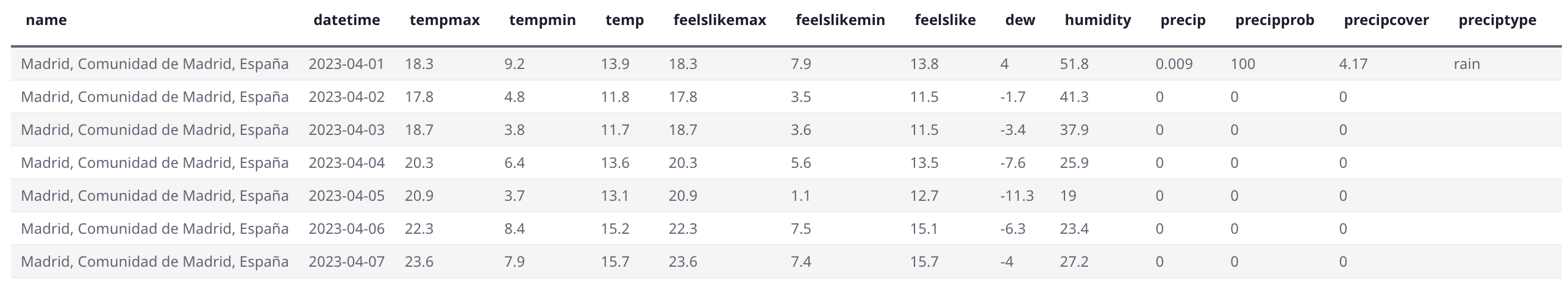
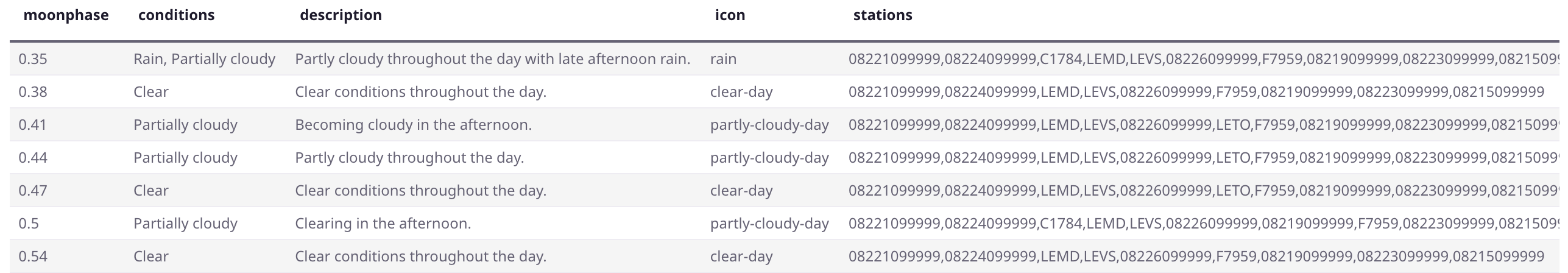
After hours of searching, I found a website where I can download historical weather data. I downloaded historical daily data from January 1st of 2016 until 25th April of 2023.
Let’s have a first look at the data:

Cleaning and Preprocessing the Data
Let’s check how many rows we have in the dataframe. As we have a little less than seven and a half years of daily data, we should have somewhat more than 2500 rows.
print(len(df))
2672
To begin with, let’s drop all the surely unnecessary columns:
df.drop(['name', 'datetime', 'temp', 'feelslikemax', 'feelslikemin', 'feelslike',
         'precipprob', 'precipcover', 'preciptype', 'snow', 'snowdepth',
         'visibility', 'solarradiation', 'solarenergy', 'uvindex', 'severerisk',
         'sunrise', 'sunset', 'moonphase', 'conditions', 'description', 'stations'],
        axis=1, inplace=True)
Now, let’s have a closer look at the data:
print(df.describe())
           tempmax      tempmin          dew     humidity       precip
count  2672.000000  2672.000000  2672.000000  2672.000000  2672.000000
mean     20.987575    10.056886     5.636265    57.654454     1.384437
std       8.912665     6.962045     4.811608    18.397388     4.716287
min       0.800000    -9.200000   -13.000000    17.000000     0.000000
25%      13.300000     4.600000     2.400000    42.675000     0.000000
50%      19.450000     9.300000     6.000000    56.500000     0.000000
75%      28.300000    15.600000     9.100000    72.100000     0.147000
max      41.300000    26.400000    17.100000    98.300000    55.173000

          windgust    windspeed      winddir  sealevelpressure   cloudcover
count  2339.000000  2672.000000  2672.000000       2671.000000  2672.000000
mean     35.342069    17.472829   168.800112       1017.646275    40.403144
std      22.121910     7.814818   111.818612          6.672164    28.249602
min       0.000000     3.800000     0.200000        987.200000     0.000000
25%      21.900000    11.400000    48.500000       1013.300000    14.600000
50%      29.500000    16.100000   202.400000       1017.100000    38.350000
75%      39.750000    22.200000   255.900000       1021.650000    64.100000
max     177.700000    55.600000   359.900000       1038.500000    98.900000
My focus is on the min, max, mean and std (standard deviation) values. They seem to be correct and consistent, it looks like there are no big outliers in the data.
It is very important to check whether you have missing values, let’s do it:
print(df.isna().sum())
tempmax               0
tempmin               0
dew                   0
humidity              0
precip                0
windgust            333
windspeed             0
winddir               0
sealevelpressure      1
cloudcover            0
icon                  0
It shows there is one line where the sea level pressure is missing, we can just delete this line. However, the wind gust value is missing for 333 lines. It’s hard to see if the measurement is missing or the values are zero. After a short research I decided to delete this column, I think the wind speed column is more relevant for us.
Dropping the windgust column:
df.drop(['windgust'], axis=1, inplace=True)
Dropping the rows that have missing (NaN) values:
df.dropna(inplace=True)
It should drop only one row, let’s double-check if indeed only one row was dropped:
print(len(df))
2671
We had 2672 rows, now we have 2671, perfect.
Now let’s check the data types of the columns in the dataframe:
print(df.dtypes)
tempmax             float64
tempmin             float64
dew                 float64
humidity            float64
precip              float64
windspeed           float64
winddir             float64
sealevelpressure    float64
cloudcover          float64
icon                 object
As expected, apart from the icon column all values are numeric, so they are okay. As machine learning models work with numbers, we have to convert the categorical icon column into several numeric columns containing 0 or 1 for each possible value.
First, let’s check the possible values of this column:
print(df['icon'].unique())
['rain' 'clear-day' 'partly-cloudy-day' 'cloudy' 'snow']
Okay, now let’s create the numeric 0/1 column for each of these values:
df = pd.get_dummies(df, columns=['icon'], dtype=np.int8)
The new columns:
print(df[['icon_clear-day', 'icon_cloudy', 'icon_partly-cloudy-day', 'icon_rain',
          'icon_snow']].head())
   icon_clear-day  icon_cloudy  icon_partly-cloudy-day  icon_rain  icon_snow
0               0            0                       0          1          0
1               0            0                       0          1          0
2               0            0                       0          1          0
3               0            0                       0          1          0
4               0            0                       0          1          0
Perfect, our data is getting cleaner and cleaner. All of our features are numeric now. The target column is still missing from the dataframe though. We need to add a new column called rain_tomorrow that will be 1 if it rained the next day or 0 if it didn’t. I will do this in several steps. First, I will add a new column called rain_today using the same logic as mentioned for rain_tomorrow. If the precipitation is more than 0 mm, then it rained that day. (It’s worth noting here that precip can mean rain or snow as well. So, even if it snowed, the rain_today column will be one. Therefore, snow will be considered as rain in our model, but anyway, it hardly ever snows in Madrid.) Then, the rain_tomorrow value will be the rain_today value from the next row. The last row will not have any value of course, so either I could drop this row, but I decided to set this value manually. Finally, I set the column type as integer.
df['rain_today'] = (df['precip'] > 0.0).astype(np.int8)
df['rain_tomorrow'] = df['rain_today'].shift(-1)
# it didn't rain on 26th April 2023
df.iloc[-1, df.columns.get_loc('rain_tomorrow')] = 0
df['rain_tomorrow'] = df['rain_tomorrow'].astype(np.int8)
The two new columns added:
print(df[['rain_today', 'rain_tomorrow']].tail())
      rain_today  rain_tomorrow
2667           0              1
2668           1              0
2669           0              0
2670           0              0
2671           0              0
Now let’s check how each column correlates to the target rain_tomorrow value. This is to see how strong the linear relationship is between the feature columns and the target.
df_corr = df.corr(method='pearson')[['rain_tomorrow']]
I use the Pearson method to calculate the correlation coefficient (Pearson’s r), which means:
- r = 1 -> strong positive linear relationship
- r = 0 -> not linearly correlated
- r = -1 -> strong negative linear relationship
Now let’s sort the values and visualize it:
df_corr.sort_values('rain_tomorrow', ascending=False, inplace=True)

plt.bar(x=df_corr.index, height=df_corr['rain_tomorrow'])
plt.xticks(rotation=90)
plt.show()
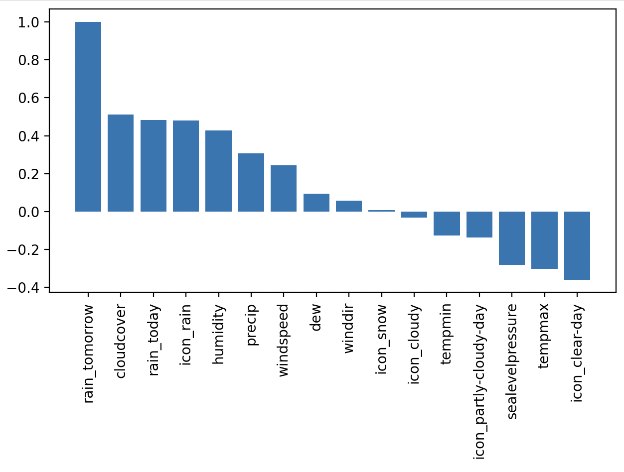
According to the result, the three columns that have the weakest linear relationship with the rain_tomorrow column are: winddir, icon_snow and icon_cloudy. The column icon_cloudy has a very weak linear relationship with rain_tomorrow, maybe it is because of the cloudcover column. Anyway, I don’t feel like removing it, let me leave it for now. I will remove winddir and icon_snow columns from the dataframe. Later I will test whether removing more features has a positive effect on the predictions.
df.drop(['winddir', 'icon_snow'], axis=1, inplace=True)
Normalizing the Data
Normalizing our data is important to ensure that the values are on a similar scale. We scale our data so that it falls within a small or specified range.
scaler = preprocessing.MinMaxScaler()
scaler.fit(df)
df = pd.DataFrame(scaler.transform(df), index=df.index, columns=df.columns)
sklearn's MinMaxScaler scales and translates each feature individually such that it is in the given range, for example between zero and one.
More about normalization techniques here.
The data after normalization:
print(df.head())
    tempmax   tempmin       dew  humidity    precip  windspeed
0  0.328395  0.477528  0.710963  0.876999  0.028655   0.339768
1  0.259259  0.376404  0.584718  0.771218  0.009062   0.401544
2  0.264198  0.311798  0.617940  0.942189  0.003154   0.496139
3  0.323457  0.477528  0.777409  0.906519  0.072753   0.878378
4  0.202469  0.407303  0.455150  0.594096  0.056259   0.482625

   sealevelpressure  cloudcover  icon_clear-day  icon_cloudy
0          0.666667    0.836198             0.0          0.0
1          0.672515    0.509606             0.0          0.0
2          0.586745    0.816987             0.0          0.0
3          0.348928    0.954499             0.0          0.0
4          0.409357    0.359960             0.0          0.0

   icon_partly-cloudy-day  icon_rain  rain_today  rain_tomorrow
0                     0.0        1.0         1.0            1.0
1                     0.0        1.0         1.0            1.0
2                     0.0        1.0         1.0            1.0
3                     0.0        1.0         1.0            1.0
4                     0.0        1.0         1.0            1.0
Splitting the Data into Training and Testing Sets
Now that we have our data cleaned up, preprocessed and normalized, we can split it into training and testing data. The machine learning model will use the training set to train the model and the testing set will be used for the evaluation of the model. You have to test your model on data it has never seen before. Sometimes our model can be overfitting, meaning that it works well for the already seen training data, but inefficient for unseen data. A good practice is to dedicate 70-75% to the training set and 25-30% to the testing set.
Also, we have to split our data into features and target. The target value is the rain_tomorrow column, this is what we are trying to predict.
Let’s see how it looks like using the sklearn's (scikit-learn) train_test_split function:
X = df.loc[:, df.columns != 'rain_tomorrow']
y = df['rain_tomorrow']

X_train, X_test, y_train, y_test = train_test_split(X, y, test_size=0.3,
                                                    stratify=y, random_state=123)
So, X gets all the columns except the target column and y gets only the target, the value to be predicted. Then, we split both into training and testing sets. The stratify parameter makes sure that the possible outcomes are represented equally in the original and the split datasets. The random_state is useful to get the same result across several executions.
Checking the effect of using stratified sampling:
print("rain_tomorrow ratio in original dataset: {}".format(
        y[y==1].count() / y.count()))
print("rain_tomorrow ratio in training dataset: {}".format(
        y_train[y_train==1].count() / y_train.count()))
print("rain_tomorrow ratio in testing dataset: {}".format(
        y_test[y_test==1].count() / y_test.count()))
rain_tomorrow ratio in original dataset: 0.35829277424185696
rain_tomorrow ratio in training dataset: 0.3584804708400214
rain_tomorrow ratio in testing dataset:  0.35785536159601
Perfect, we have split our data, it’s time to build some models.
Which model(s) to use?
First of all, let’s lay down some facts.
We are building a supervised machine learning model. In a nutshell, supervised learning is when we work on known and previously labelled data. For example, to predict the weather based on historical data, to predict property prices based on size, neighborhood, etc, to decide if an image is a dog or a cat or for example in medicine to decide the type of a tumor. Unsupervised learning is when we group unlabelled data. For example, grouping people based on their market activity or grouping users based on their activity. Our task at hand clearly requires a supervised machine learning algorithm.
Supervised machine learning algorithms can be divided into two categories: classification and regression. Classification is used to assign data into specific categories. For example, classify images based on the animal they have or classify medical tumors. Regression is used to predict a continuous variable, such as income, price, temperature or number of something. In case of regression there is a relationship between the dependent (target) and independent (features) variables. A linear regression model could be used for instance to predict the number of car rentals a day or the price of a property.
Now, let’s see how three different models perform to solve our task.
Solution 1 - Logistic Regression
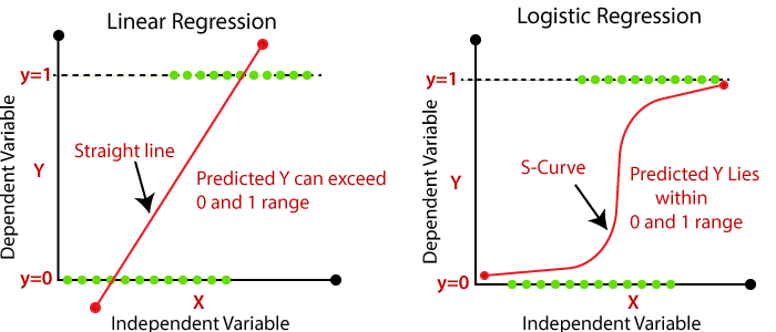
In linear regression, when the dependent variable is categorical and has binary outputs (0 or 1, True or False), then it is a logistic regression. Logistic regression is basically used to solve binary classification problems such as whether an email is spam or not. And yes, it can be used for our problem as well: whether it will rain tomorrow or not. The image below reflects quite well the difference between linear and logistic regression. We could say that in case of logistic regression the continuous variable can have only two values.
Let’s see how this looks like in Python using LogisticRegression from the sklearn library. I will provide the random_state variable to always get the same result, apart from that I will just use the default parameters.
log_reg = LogisticRegression(random_state=123)
log_reg.fit(X_train, y_train)

x_pred = log_reg.predict(X_train)
score = accuracy_score(y_train, x_pred)
print("Prediction score for training data: {}".format(score))

y_pred = log_reg.predict(X_test)
score = accuracy_score(y_test, y_pred)
print("Prediction score for test data: {}".format(score))

print(classification_report(y_pred, y_test))
Prediction score for training data: 0.7929373996789727
Prediction score for test data: 0.773067331670823
              precision    recall  f1-score   support

         0.0       0.90      0.78      0.84       589
         1.0       0.55      0.75      0.64       213

    accuracy                           0.77       802
   macro avg       0.72      0.76      0.74       802
weighted avg       0.80      0.77      0.78       802
We create a LogisticRegression model object and call the fit() method to train the algorithm on the training data. Then we make predictions for our training data as well as for our testing data and print out the score. The accuracy of our predictions is around 79% for the training data and around 77% for the testing data. I also print out the classification report where we can get a more detailed evaluation. As we can see, the model is 90% accurate to predict no rain, but only 55% accurate to predict rain for tomorrow. There is room to improve.
Solution 2 - Decision Tree
The second algorithm I want to try is the decision tree. Decision trees can be used to solve both classification and regression problems. They start with a root node that can have outgoing branches which feed into decision nodes. It ends with terminal nodes that represent the possible outcomes. The depth of the decision tree is important to be set right, otherwise our model can be overfitting or underfitting. Decision trees are created by recursive partitioning, where the data is split into partitions. This ends when: all the data in the partition are of the same class; the specified tree limit size has been met; or all features have been exhausted. There are several ways to measure the impurity of the tree, sklearn's DecisionTreeClassifier uses Gini by default.
To begin with, let’s run a decision tree model without setting any parameter:
dtc = DecisionTreeClassifier(random_state=123)
dtc.fit(X_train, y_train)

x_pred = dtc.predict(X_train)
score = accuracy_score(y_train, x_pred)
print("Prediction score for training data: {}".format(score))
y_pred = dtc.predict(X_test)
score = accuracy_score(y_test, y_pred)
print("Prediction score for test data: {}".format(score))
Prediction score for training data: 1.0
Prediction score for test data: 0.6895261845386533
As we can see, the model is overfitting, meaning that it works perfectly with the training data, but poorly with the test data.
Now let’s “play” with some parameters. Using sklearn's GridSearchCV class we can run an exhaustive search over a set of predefined parameter values. Then, having found the best combination of parameters we can build and train the decision tree model.
dtc = DecisionTreeClassifier(random_state=123)
param_grid = {'max_depth': [3, 4, 5, 6],
              'min_samples_split': [2, 3, 5, 10],
              'min_samples_leaf': [1, 2, 3, 5],
              # 'criterion': ['gini', 'entropy', 'log_loss']}
gs = GridSearchCV(estimator=dtc, param_grid=param_grid)
gs.fit(X_train, y_train)
dtc = gs.best_estimator_
print("best model: {}".format(dtc))
dtc.fit(X_train, y_train)

x_pred = dtc.predict(X_train)
score = accuracy_score(y_train, x_pred)
print("Prediction score for training data: {}".format(score))
y_pred = dtc.predict(X_test)
score = accuracy_score(y_test, y_pred)
print("Prediction score for test data: {}".format(score))

print(classification_report(y_pred, y_test))
best model: DecisionTreeClassifier(max_depth=3, random_state=123)
Prediction score for training data: 0.7849117174959872
Prediction score for test data: 0.7755610972568578
              precision    recall  f1-score   support

         0.0       0.90      0.78      0.84       593
         1.0       0.55      0.76      0.64       209

    accuracy                           0.78       802
   macro avg       0.73      0.77      0.74       802
weighted avg       0.81      0.78      0.79       802
Well, the result is more or less the same as that of the logistic regression. We are pretty good to predict no rain, but only 55% accurate to predict rain. As you can see the commented line in the param_grid dictionary, I also tried several methods to measure the quality of the split during the partitioning process, but I didn’t get better results. One reason can be definitely the lack of sufficient data, but I’ll check some things later regarding this.
Before we move on, I want to show you how you can plot your actual decision tree model. Based on the tree we can also have some clues what to change in our parameters.
plot_tree(dtc, feature_names=list(X.columns), class_names=True, filled=True)
plt.show()

As shown, if the cloudcover is less than a certain value, the prediction will be always 0, no matter what. I have done some tests removing this column and/or others, but I didn’t get better results than the one above.
Solution 3 - Gradient Boosting Classifier
The first two solutions are quite “well-known”, however, this third option that I will try was new to me until I saw it in a LinkedIn course. Then I made some research and thought I would try it. It’s the gradient boosting classifier: “it is a group of machine learning algorithms that combine many weak learning models together to create a strong predictive model. Decision trees are usually used when doing gradient boosting. Gradient boosting models are becoming popular because of their effectiveness at classifying complex datasets.”
We will use sklearn's GradientBoostingClassifier in the following example.
gbc = GradientBoostingClassifier()
param_grid = {'n_estimators': [100, 200, 500],
              'max_depth': [3, 5, 6],
              'min_samples_leaf': [1, 5, 10, 15],
              'loss': ['log_loss']}
gs = GridSearchCV(gbc, param_grid=param_grid, n_jobs=4)
gs.fit(X_train, y_train)
gbc = gs.best_estimator_
print("best model: {}".format(gbc))
gbc.fit(X_train, y_train)

x_pred = gbc.predict(X_train)
score = accuracy_score(y_train, x_pred)
print("Prediction score for training data: {}".format(score))
y_pred = gbc.predict(X_test)
score = accuracy_score(y_test, y_pred)
print("Prediction score for test data: {}".format(score))

print(classification_report(y_pred, y_test))
best model: GradientBoostingClassifier(min_samples_leaf=15)
Prediction score for training data: 0.8533975387907973
Prediction score for test data: 0.7618453865336658
              precision    recall  f1-score   support

         0.0       0.88      0.78      0.83       578
         1.0       0.56      0.71      0.63       224

    accuracy                           0.76       802
   macro avg       0.72      0.75      0.73       802
weighted avg       0.79      0.76      0.77       802
You may note that I’m using GridSearchCV again to find the optimal parameters. As we can see, the accuracy is almost the same as in the previous two solutions. Almost 80% on the test data is not so bad, however, only 56% correct on predicting rain. We should do better.
Let’s analyse the results and see what we can do.
Analyzing Results
All three solutions have more or less the same results. An overall accuracy of around 80% on the test data, where we have around 90% accuracy of predicting no rain and 55% accuracy of predicting rain. We have to emphasize the fact that we have quite little data and among this data rainy records are underrepresented. It shouldn’t be a surprise either in Madrid, where we talk about 300+ sunny days per year. Probably this is one of the reasons why our models are more accurate on predicting no rain. Also, it would be worth “playing” with the features. Sometimes less features are more effective, useless features can even do harm to the model. And maybe most importantly, gathering more data could give a big push to achieve better results. Having sufficient data, quantity as well as quality, is key to a successful machine learning model. These mentioned points will be my next steps.
Also, this is my first ever machine learning project, it would be useful to hear some advice from experienced machine learning engineers.
After Gathering More Data
I have downloaded more historical weather data so now I have more than 6300 rows of data, dating from 1st January of 2006 until 25th April of 2023.
Having more data, running the same models gave me much better results.
Logistic Regression
Prediction score for training data: 0.7921373700858563
Prediction score for test data: 0.7970479704797048
              precision    recall  f1-score   support

         0.0       0.86      0.81      0.84      1217
         1.0       0.70      0.77      0.73       680

    accuracy                           0.80      1897
   macro avg       0.78      0.79      0.78      1897
weighted avg       0.80      0.80      0.80      1897
The logistic regression model gave me 80% overall accuracy, slightly more than before, however, this time we have 70% accuracy of predicting rain. This is a big improvement from the 55% before. And doing nothing, only having more data. I have tried deleting some features, but couldn’t get a better result.
Decision Tree
best model: DecisionTreeClassifier(max_depth=4, random_state=123)
Prediction score for training data: 0.7855851784907365
Prediction score for test data: 0.7796520822351081
              precision    recall  f1-score   support

         0.0       0.85      0.80      0.82      1212
         1.0       0.68      0.74      0.71       685

    accuracy                           0.78      1897
   macro avg       0.76      0.77      0.77      1897
weighted avg       0.79      0.78      0.78      1897
Just like in case of the logistic regression, the decision tree model also gave me a better result. The overall accuracy stayed almost the same, but the accuracy to predict no rain went up to 68%. Also, if you notice, having more data had on effect on the parameters. The optimal max_depth is now four instead of three.
It is worth noting here that when you create and optimize your model, it may not be the final version. When/if you have more or different data, you have to adjust your model as well.
Gradient Boosting Classifier
gbc = GradientBoostingClassifier()
param_grid = {'n_estimators': [100, 200, 500],
              'max_depth': [3, 4, 5],
              'min_samples_leaf': [7, 10, 12],
              'loss': ['log_loss']}
gs = GridSearchCV(gbc, param_grid=param_grid, n_jobs=4)
gs.fit(X_train, y_train)
gbc = gs.best_estimator_
print("best model: {}".format(gbc))
gbc.fit(X_train, y_train)

x_pred = gbc.predict(X_train)
score = accuracy_score(y_train, x_pred)
print("Prediction score for training data: {}".format(score))
y_pred = gbc.predict(X_test)
score = accuracy_score(y_test, y_pred)
print("Prediction score for test data: {}".format(score))

print(classification_report(y_pred, y_test))
best model: GradientBoostingClassifier(max_depth=4, min_samples_leaf=10)
Prediction score for training data: 0.8398102123813828
Prediction score for test data: 0.7959936742224565
              precision    recall  f1-score   support

         0.0       0.85      0.82      0.83      1183
         1.0       0.72      0.75      0.74       714

    accuracy                           0.80      1897
   macro avg       0.78      0.79      0.78      1897
weighted avg       0.80      0.80      0.80      1897
After changing a little the hyperparameters, I found the above as the best result I can get. Not bad. 85% accuracy of predicting no rain and 72% accuracy of predicting rain. The former is the same as the decision tree model, although the latter is way better.
It is interesting to see the behavior of the models. Depending on the data different models performed better. It’s advised to always try different models and see which performs the best.
After Dropping More Features
Looking again at the feature importances of the models, I decided to delete the icon column from the dataframe. The feature importance shows how useful a feature is to predict the target variable.
# Logistic Regression
importance = log_reg.coef_[0]
feature_importance = pd.Series(importance, index=X_train.columns)
feature_importance.sort_values().plot(kind='bar')
plt.ylabel('Importance')
plt.show()

# Decision Tree
importance = dtc.feature_importances_
feature_importance = pd.Series(importance, index=X_train.columns)
feature_importance.sort_values().plot(kind='bar')
plt.ylabel('Importance')
plt.show()
It clearly showed that the icon_* columns are not useful.
After dropping the icon column I got an around 1% better result with all the models. It is advised to remove useless features because they can even harm the model.
Conclusions
Having carried out this exercise full of learning and fun, my main conclusion is that implementing the machine learning models, actually writing those few lines is the least concern of all. In my opinion the most important is to actually know the models, to know what plays out “behind the scenes” and to be able to choose the right model. Just as important it is to have good data. Sufficient quantity, quality and variety. We have seen clearly that just by having more data we could achieve a much more accurate result. Basically we could detect the same tendency for all models. The more data we had, the more accurate the model was. And as the data changed, we may have had to adapt our models as well.
I’m really happy to have completed this first journey with machine learning, this is the first of more to come. I have found it very exciting and have enjoyed every minute of it. I have to confess that after completing more than 15 hours of courses and having read about the topic, I was hungry for some action.
Well, thanks for reading, time for me to sleep.
This blog post provides a clear explanation of how machine learning can predict rainfall.
ReplyDelete