
One of the greatest things in life for me is definitely travelling. People who travel with me know that I take a lot of photos. These photos have turned out to be quite handy for my new machine learning project to classify images.
The Goal
Using Python’s Keras library, I want to build a neural network and train it on my travelling photos to classify images whether they contain any water or not. Any water such as sea, ocean, river, lake, etc.
The Image Dataset
First of all, we need to manually classify the photos to be used to train the model. In order to make this process easier and faster, I wrote a simple Python script to do so. In brief, it displays all of the images from the source folder and based on the key that we press it copies the image into the specific category folder.
My image dataset has 740 photos from several countries representing seas, rivers and lakes in various light conditions.
The Solution
You can find the source code on GitHub.
I use Python’s Keras which is a deep learning API built on top of TensorFlow. It simplifies the process of creating and training neural networks.
Loading the images into the training and validation datasets
Keras provides a quite handy function that loads all images from a source folder and classifies them based on the subfolder they are in.
train_ds, val_ds = keras.utils.image_dataset_from_directory(
	IMAGES_PATH,
	labels="inferred",
	color_mode="rgb",
	batch_size=10,
	image_size=(256, 256),
	shuffle=True,
	validation_split=0.2,
	subset="both",
	seed=123,
	label_mode="binary"
)

class_names = np.array(train_ds.class_names)
print(class_names)
Found 740 files belonging to 2 classes.
Using 592 files for training.
Using 148 files for validation.
['other' 'water']
All 740 images were loaded and labelled based on the two subfolders, water and other.
Making sure that the datasets have the expected shapes:
[(image_batch, label_batch)] = train_ds.take(1)
print(image_batch.shape)
print(label_batch.shape)
(10, 256, 256, 3)
(10, 1)
The image_batch represents the features of the image data. We have 10 images per batch, 256x256 is the size in pixels and 3 is for the RGB channels. The labels have 10 images per batch too and one target column to mark the category.
Rescaling the data
RGB channels are in the [0-255] range which is not ideal for neural networks, so we need to standardize these to be within the [0-1] range.
rescaling_layer = keras.layers.Rescaling(1.0 / 255)
train_ds = train_ds.map(lambda x, y: (rescaling_layer(x), y))
val_ds = val_ds.map(lambda x, y: (rescaling_layer(x), y))
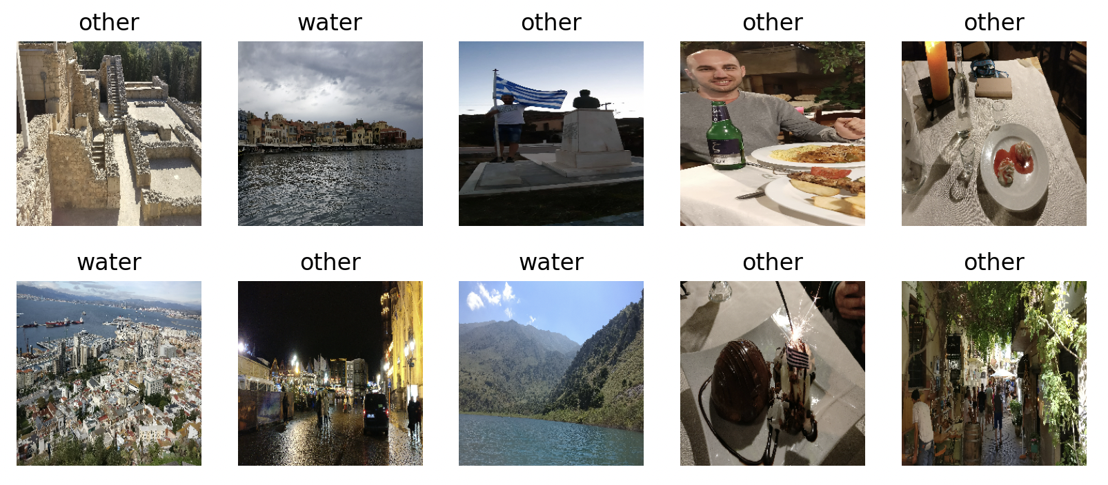
Displaying some examples
Let’s display ten photos from the image dataset to have a clue about our data.
for image_batch, label_batch in train_ds.take(1):
	plt.figure(figsize=(10, 4))
	plt.subplots_adjust(hspace=0.3)
	for n in range(10):
		plt.subplot(2, 5, n+1)
		plt.imshow(image_batch[n])
		plt.title(class_names[int(keras.backend.get_value(label_batch[n])[0])])
		plt.axis('off')
plt.show()
Prefetching to improve the performance
train_ds = train_ds.cache().prefetch(buffer_size=tf.data.AUTOTUNE)
val_ds = val_ds.cache().prefetch(buffer_size=tf.data.AUTOTUNE)
Prefetching uses a background thread and an internal buffer to prefetch elements from the input dataset ahead of the time they are requested.
Building the model
model = keras.models.Sequential()

model.add(keras.layers.Conv2D(filters=32,
                              # number of filters in the layer; each filter will
                              # be able to detect one pattern in the image
							  kernel_size=(3, 3),
							  # size of the window that we'll use when creating
							  # image tiles from each image; 3 x 3 pixels
							  padding="same",
							  # if in the last image tile we don't have 3 pixels
							  # left, we pad it with zeros
							  input_shape=(256, 256, 3),
							  # 256 pixels x 256 pixels and 3 RGB channels
							  # input shape required only for the first layer
							  activation="relu" # activation function
							  )
          )
model.add(keras.layers.MaxPooling2D(pool_size=(2, 2)))
model.add(keras.layers.Dropout(0.25))

model.add(keras.layers.Conv2D(64, (3, 3), padding="same", activation="relu"))
model.add(keras.layers.MaxPooling2D(pool_size=(2, 2)))
model.add(keras.layers.Dropout(0.25))

model.add(keras.layers.Flatten())
model.add(keras.layers.Dense(512, activation="relu"))
model.add(keras.layers.Dropout(0.5))
model.add(keras.layers.Dense(1, activation="sigmoid"))
We create a sequential model that indicates to Keras that each layer that we add to the neural network is the input of the next layer.
Objects normally are not always in the centre of the image, they can be at any place and have variable sizes. To tackle this challenge we use convolutional layers. As we work with images, it is two-dimensional.
The max pooling layer is used to make the model more efficient by downsampling the input data to keep the most useful data only. If the pool size is (2, 2), it means we take 2x2, four pixels and take the maximum.
The dropout layer forces the neural network to learn and not to memorize the data. We drop a certain percentage of the connections (normally between 25 and 50) in order to avoid overfitting the training dataset.
The flatten layer flattens the dimensions after the convolutional layers. This is required when we transition to the dense layer.
The dense layer is deeply connected to the preceding layer, meaning all of its neurons are connected to each neuron of the preceding layer. The output of the dense layer is specified by the parameter. The last dense layer is the output layer and in our case it has one node as we have a binary classification. If we had ten possible output categories, it should have ten output nodes.
model.compile(
	loss="binary_crossentropy",
	optimizer=keras.optimizers.legacy.Adam(),
	metrics=["acc"]
)
By compiling the model we configure it for the training.
The loss function is used to calculate how far the neural network’s guesses are from the actual value. For more than two classes we’d use categorical_crossentropy.
The optimizer parameter tells Keras which optimization algorithm to use during the training. This is to update the weights of the neural network after calculating the difference between the predicted and actual values of the model.
At last we define the list of metrics to be evaluated by the model during training and testing.
Model summary output:
model.summary()
Model: "sequential"
_________________________________________________________________
 Layer (type)                Output Shape              Param #
=================================================================
 conv2d (Conv2D)             (None, 256, 256, 32)      896

 max_pooling2d (MaxPooling2  (None, 128, 128, 32)      0
 D)

 dropout (Dropout)           (None, 128, 128, 32)      0

 conv2d_1 (Conv2D)           (None, 128, 128, 64)      18496

 max_pooling2d_1 (MaxPoolin  (None, 64, 64, 64)        0
 g2D)

 dropout_1 (Dropout)         (None, 64, 64, 64)        0

 flatten (Flatten)           (None, 262144)            0

 dense (Dense)               (None, 512)               134218240

 dropout_2 (Dropout)         (None, 512)               0

 dense_1 (Dense)             (None, 1)                 513

=================================================================
Total params: 134238145 (512.08 MB)
Trainable params: 134238145 (512.08 MB)
Non-trainable params: 0 (0.00 Byte)
_________________________________________________________________
We can see a summary of the layers in our model and it displays the number of parameters as well. The trainable parameters are the ones that the neural network has to learn during the training process. Check here how it is calculated in detail.
The actual training of the model happens when we fit the model.
model.fit(
	train_ds,
	epochs=5,
	validation_data=val_ds,
	shuffle=True
)
The epochs parameter sets how many times we want to go through our training dataset during the process. This is an important parameter. The more epochs, the more chance our model has to learn. But if too many, our model may not learn anything new and just run in vain or even lose accuracy. For very large datasets five epochs can be a good start. I set it as five in my example, because the way I saw it didn’t really learn anything new after those five epochs. The batch_size parameter sets how many images to feed into the network at once. Lower value means longer training, higher means more memory consumption. Usually it is between 32 and 128. As our dataset is already batched, we don’t need to specify it.
Epoch 1/5
60/60 [==============================] - 29s 455ms/step - loss: 2.9112 - acc: 0.6351 - val_loss: 0.5896 - val_acc: 0.6892
Epoch 2/5
60/60 [==============================] - 19s 307ms/step - loss: 0.4993 - acc: 0.7821 - val_loss: 0.4875 - val_acc: 0.7230
Epoch 3/5
60/60 [==============================] - 18s 308ms/step - loss: 0.4434 - acc: 0.8142 - val_loss: 0.4989 - val_acc: 0.7500
Epoch 4/5
60/60 [==============================] - 19s 310ms/step - loss: 0.3472 - acc: 0.8581 - val_loss: 0.5077 - val_acc: 0.6959
Epoch 5/5
60/60 [==============================] - 19s 310ms/step - loss: 0.2415 - acc: 0.8986 - val_loss: 0.4460 - val_acc: 0.7905
We got an accuracy of about 79%. We’ll see how it performs on images the model has never been before.
Saving the model
We save our model into the default TensorFlow SavedModel format so that we don’t have to train it each and every time. Training a model can take minutes, but also hours, days or even weeks.
model.save("saved_model")
Validation
Now let’s validate the model with twenty photos it has never seen before. The tfk_predict_water library loads the previously saved model and displays the twenty images with the predictions. You can check the full code on GitHub.
plt.figure(figsize=(10, 10))
plt.subplots_adjust(hspace=0.5)
n = 0
for image_file in os.listdir(IMAGES_PATH):
	if image_file.split('.')[-1].lower() != 'jpg':
		continue
	img = image.load_img(os.path.join(IMAGES_PATH, image_file),
	                     target_size=(256, 256))
	image_to_test = image.img_to_array(img)
	results = model.predict(np.expand_dims(image_to_test, axis=0))
	result = results[0]
	class_label = CLASS_LABELS[int(result)]
	plt.subplot(5, 5, n+1)
	plt.imshow(image_to_test/255)
	plt.title(class_label)
	plt.axis('off')
	n += 1
plt.show()
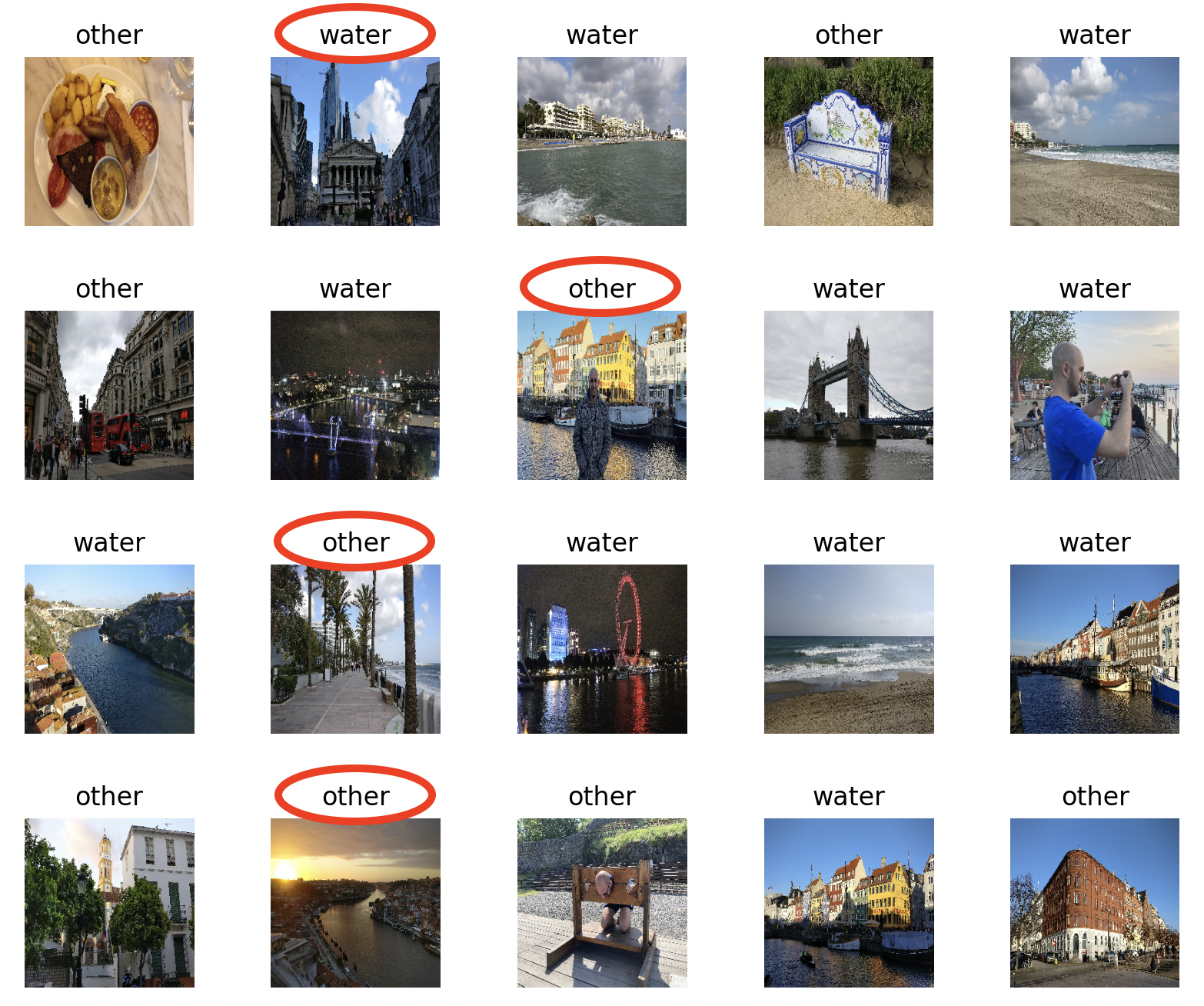
As we can see, the model is not too bad to start with, but clearly it needs much more photos to be trained on. Sometimes the result is surprisingly good, for example the photos in the last column of the first and second rows. However, the model performs poorly for the marked photos in the second and fourth row.
Also, I want to note that after several tests I got somewhat different results, but the incorrect guesses were consistently between four and seven. I “played” with the batch number as well, it seemed to me like it works best between 10 and 20.
These are the results of other executions:


We can see some photos are consistently misclassified.
Conclusion
I might have aimed a little high with my goal to recognize images with water on them. Also, obviously, we would need much more photos to train a better model. Probably it would have been “easier” to recognize cars or objects whose form and shape don’t change substantially. All things considered, I think the above result is not so bad to start with, especially because of the relatively small number of images I used for training the model.
Anyway, I have a great challenge at hand and I will not stop until having all of my travelling photos classified. Until then, more learning and much more travelling to come …
Comments
Post a Comment